Code Checkpoints

Research · November 2, 2026

Driving Made Simple: A Fully Open Recipe from Public Data

Open-weight models are advancing the capabilities of autonomous systems over a broad set of domains^[1][2]. In the LLM and robotics communities, open-weight models have helped accelerate progress by enabling researchers to build on shared foundations, setting an encouraging example for autonomous driving^[3], where model weights have traditionally remained closed. However, even with open weights, high data and compute costs as well as closed training recipes limit reproducibility, slowing down the community's efforts to address a model's limitations.

NVIDIA's Alpamayo 1, for example, releases weights and inference code, but neither its 80,000 hours of curated proprietary training data, likely selected from more than a million hours of driving, nor its training recipe^[3]. In contrast, fully open models with open recipe releases, which include data, code, models, and evaluations, are playing an important role in enabling research progress^[4][5][6]. Unfortunately, in driving, existing fully open models have a different limitation: they are specialists, models which either only use a single benchmark or require independently tuned weights for each benchmark^[7][8]. Today, we change this. We are releasing our first fully open recipe for end-to-end driving:

General and fully open pipeline: Developed with minimal assumptions about the model architecture or the target benchmarks, our three-stage training pipeline effectively tackles two key challenges in training driving policies, the copycat problem^[9][10] and the target point bias^[11][12].
Efficient infrastructure: The complete training runs on a single 8×H100 node in under a day. One command evaluates a checkpoint on six different driving benchmarks.
The experiments behind the release: We share an open research log of more than 50 experiments. Importantly, we also include the experiments that failed.
A strong, reproducible baseline: Trained exclusively on public data and evaluated on six benchmarks, our baseline model achieves competitive performance across all of them (Figure 1, details in Appendix A).

Figure 1. A single open model, trained on public data in under a day, performs on par with the best published policies trained under the same conditions (only imitation of human driving, without closed-loop fine-tuning or benchmark-specific tuning) across six benchmarks. Left: our recipe release in py123d_garage v0.2 compared with NVIDIA’s Alpamayo 1. Right: our policy, with the same weights on every benchmark, against the best such policy per benchmark, each on its own metric, 0 to 100, higher is better. Details in Table 1.

A training recipe against shortcut learning

Central to our experiments is a camera-only Latent TransFuser^[13] with a diffusion transformer as motion planner (Figure 2). As input, the policy receives the front camera of the current timestep and one second earlier, the ego speed and, optionally, target points 40 m, 60 m and 80 m ahead on the intended route. We train on about 1,800 hours of public driving data (Table 13): the Physical AI AV dataset^[14] (about 1,650 hours), the camera subset of nuPlan^[15] (about 124 hours) and the NuRec training scenes of AlpaSim (about 7 hours).

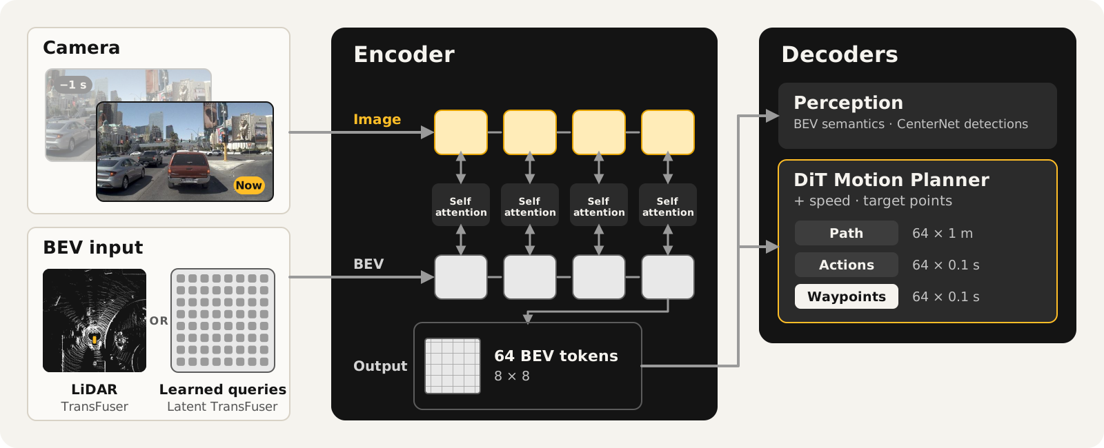
Latent TransFuser architecture: a camera branch and a BEV branch of learned queries fused by transformers at four resolutions, an output of 64 BEV tokens, and the decoders for perception and motion planning — **Figure 2.** Latent TransFuser. The current and the past front-camera frame are stacked into one image. The model also supports LiDAR input, but we do not use it here, because not all six benchmarks provide LiDAR and one policy should run on all of them. The BEV (bird's-eye view) branch starts from learned queries, and the encoder outputs 64 BEV tokens. The motion planner reads them, the ego speed and the optional target points.

Training a driving policy end-to-end is notoriously difficult, and much of the difficulty comes from shortcut learning^[16]. A policy takes the easiest path to minimizing its training loss, and unless this is done carefully, the policy can lean on cues that are unreliable at test time. In driving, two cues make shortcut learning highly likely. The first is the target points: following them is easier than interpreting the sensory inputs, so the policy steers toward them even when a point lies off the road, a phenomenon studied thoroughly in our prior work^[11][12]. The second is the ego speed: driving data consists mostly of nominal driving, where extrapolating the current speed explains most of the future speed. A policy that learns this keeps its speed instead of reacting to the scene, and brakes too late when the car ahead slows down. This is typically referred to as the inertia or copycat problem, and has been observed consistently since the pioneering research on end-to-end driving policies^[10].

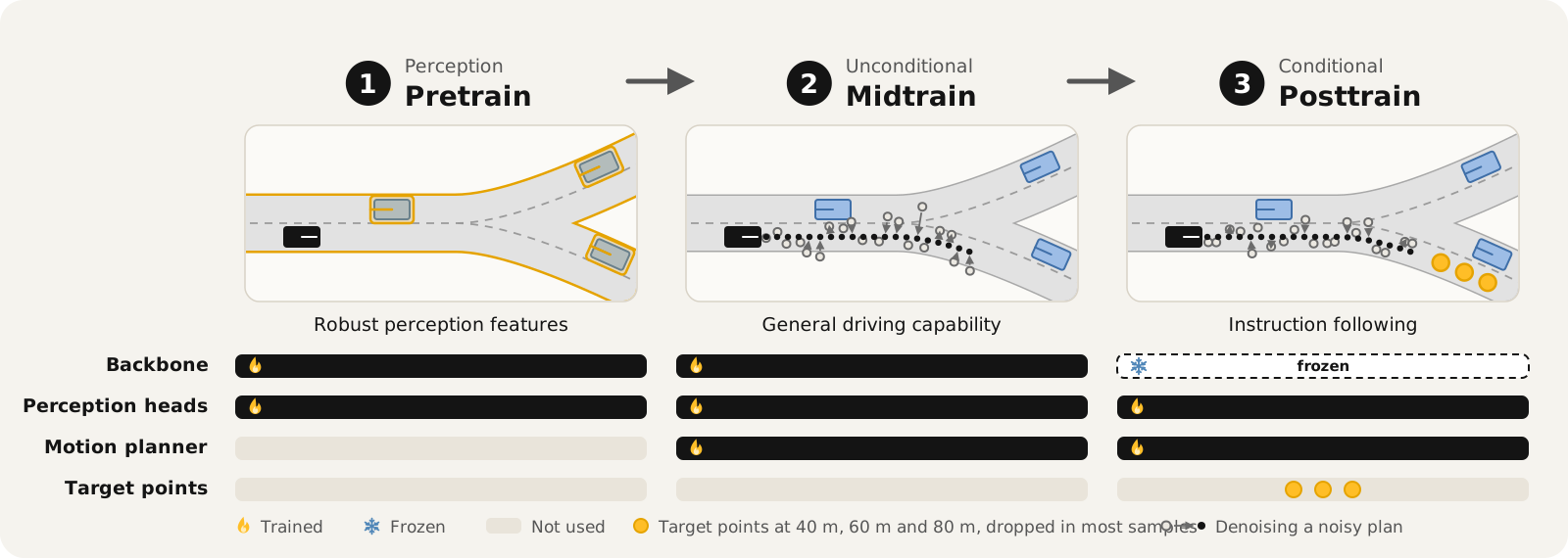
To tackle these two shortcuts, we decompose training into three stages (Figure 3). The two inputs that enable these shortcuts, the ego speed and the target points, are added only in later stages, after the network has learned to perform the perception and driving without them. In pretraining, the network focuses on learning robust perception features, making the policy interpret its sensory inputs. In midtraining, a planning decoder with access to the current vehicle speed is attached to the output of the pretrained encoder, and the policy learns general driving without target points to follow. In the final posttraining stage, target points are provided to the planner, so the policy learns to follow an instruction in addition to the driving capability it already has.

The three training stages side by side. Pretrain learns perception from BEV segmentation and boxes, midtrain picks a branch of the fork from the scene alone, posttrain follows target points with the backbone frozen. Trained parts carry a flame, the frozen backbone a snowflake. — **Figure 3.** The three training stages, each initialized with the weights of the previous stage.

Four elements are central to our recipe, as evidenced by our experiments (Figure 4, details in Appendix B):

Diffusion planning loss. A regression loss averages its output when several outputs are correct. Without target points in midtraining, this ambiguity arises at intersections and forks, where the human driver could take several different paths, and the averaged path runs between the lanes. A diffusion transformer trained with flow matching^[17] can in principle learn all of them in training and commit to one at test time. This makes the policy mode-seeking instead of mean-seeking.
Three training stages. Training the planner first without target points (midtraining) and only afterward with them (posttraining) works better than providing target points to the planner from the start (same compute budget).
Target point dropout. During posttraining, we drop each target point with a probability of 91 %, so 75 % of the training samples contain no target point and the planner still has to drive from the sensory inputs alone. The target points thereby remain an auxiliary cue that resolves ambiguities such as forks, rather than a signal the policy can directly copy.
Temporal input. A single frame carries no motion information. Hence, the planner can only infer the dynamics of the scene from the ego speed, which reinforces the inertia shortcut. Stacking the front-camera frame from one second earlier exposes the relative motion of surrounding traffic and reduces collisions.

Figure 4. Gain of each recipe choice in AlpaSim score points over the alternative, mean of three seeds. Error bars: standard deviation over the three seeds. Details in Appendix B.

Real progress should hold across benchmarks

The hidden test sets of the AlpaSim challenge^[18], which we co-organize with NVIDIA and OpenDriveLab, are unseen by policies trained only on public data. The challenge offers two tracks, nuPlan and Physical AI, with two different private test datasets. Their scenes are not released to participants, including us as co-organizers, and submissions are scored by the challenge server. A strong baseline on the Physical AI test set is Alpamayo 1^[3], NVIDIA’s 10B parameter policy trained on 80,000 hours of internal driving data, far more than is publicly available and recorded by the same fleet as the test scenes. Our 68M parameter policy is trained on 1,800 hours of public driving data.

During the development of our policies, we observed that checkpoints that did well on the validation scenes of only one of the two AlpaSim tracks underperformed Alpamayo 1 on the hidden test set of the Physical AI track. Only after combining all four elements of the training recipe (Figure 4) did we obtain a policy that does well on the public validation scenes of both nuPlan and Physical AI at the same time, and achieves a higher score than Alpamayo 1 on the hidden Physical AI test set (Figure 5).

Figure 5. Three submissions to the Physical AI track of the official AlpaSim challenge leaderboard (hidden test set), one seed each. Validation scores are computed locally on the public validation scenes, in our development setting of the time. All scores are scene scores, 0 to 100.

The general lesson: a policy that drives well only on one benchmark may just have specialized to that benchmark’s metrics. Most prior work evaluates one architecture on a single or a small set of benchmarks and retrains or tunes it for each. In contrast, we evaluate one checkpoint, unchanged, on six independent benchmarks: both AlpaSim tracks, Odyssey^[19], HUGSIM^[20], and NAVSIM^[21] v1 and v2^[22] (Figure 1, right; per-benchmark results in Table 1). Our policy scores higher than the best published policy trained under the same conditions (trained only to imitate human driving, without closed-loop fine-tuning or benchmark-specific tuning) on both AlpaSim tracks, on par on HUGSIM, and lower on Odyssey and NAVSIM.

Gains that hold across all six benchmarks are more likely to reflect better driving. This is the premise of the common task framework behind the AlpaSim challenge, and we will extend our evaluation as further independent benchmarks with held-out test sets become available.

Learning to drive in a day

Our training code allows others to reproduce our numbers and build on them without a large compute budget. The full recipe trains three seeds in 21 hours on one node with eight H100 GPUs. Two techniques, with minimal assumptions about the underlying architecture, make this affordable:

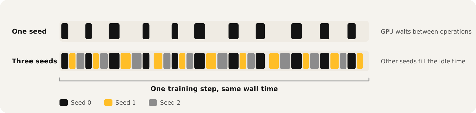
Three seeds in one training session. A 68M parameter model cannot utilize a GPU like the H100 at its full potential. This is in particular a problem since, in our experience, driving policies have always had trouble scaling with batch size under the limited scale and diversity of public driving datasets. Our release tackles this issue by fitting three seeds into one training session (Figure 6). Multiple seeds are essential for reliable conclusions: closed-loop scores vary by about 3 points from seed to seed on the Physical AI track, and now and then one seed converges to a lower score than the others, so every number in this post, except the leaderboard submissions, is a mean of three training seeds.

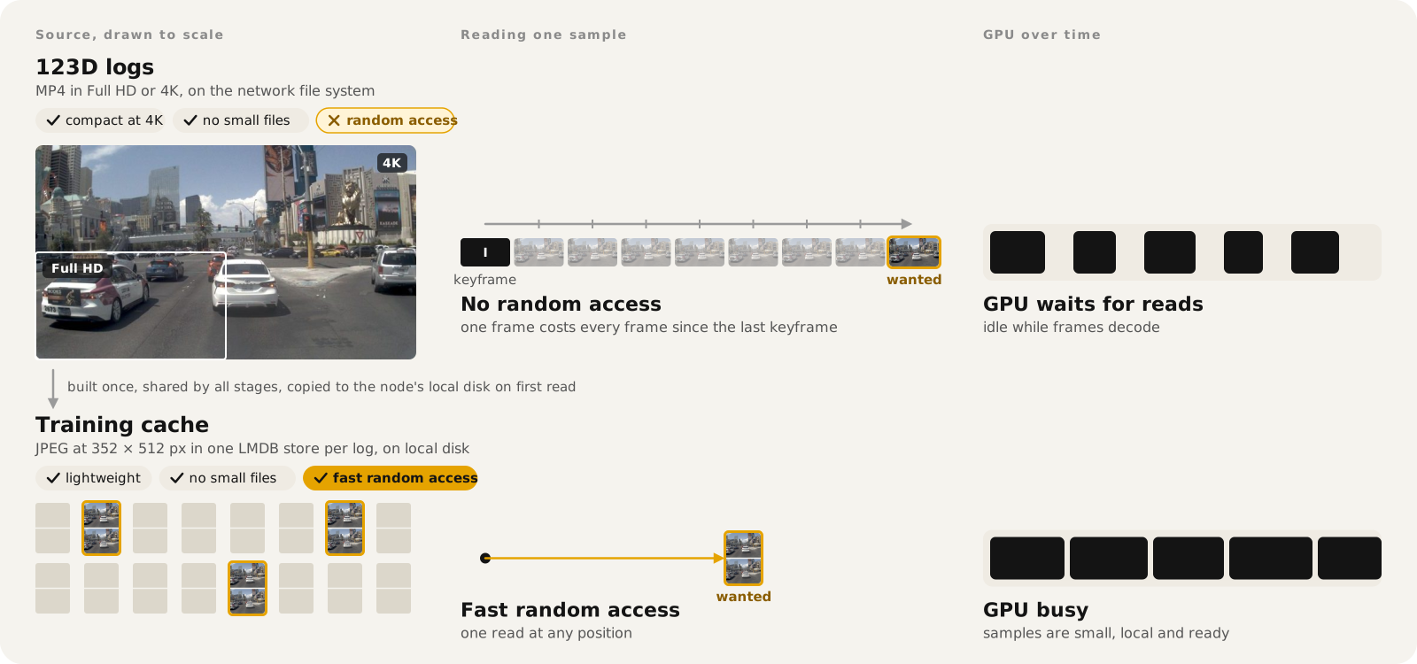
GPU timeline of one training step: with one seed the GPU waits between operations, with three seeds the operations of the other seeds fill the idle time at the same wall time per step — **Figure 6.** One training step, schematic. The three seeds share the GPU but nothing else: each has its own weights and its own third of every batch, so it trains exactly as it would alone.

Combining compact logs with lightweight training caches. py123D^[23] stores cameras as MP4 streams. At 1,800 hours of driving this is a necessity rather than a convenience: compressed video keeps the logs small enough to store, copy and share. Policy training, however, samples individual frames in random order, and reading one frame from an MP4 requires decoding every frame since the last keyframe. Our release therefore introduces a flexible cache system, built on LMDB^[24], that allows random-access training from a lightweight cache (Figure 7). It scales with the logs: one store per log lets the cache build in parallel, and one file per log instead of millions of small ones avoids hitting the file system’s limit on the number of files.

Figure 7. The training cache is built once and shared by all three training stages. Each sample is copied from the shared network storage to the local disk of the node on its first read, so all later reads come from the local disk.

Conclusion

Two lessons stood out while building this release:

Shortcut learning. As in our previous work in CARLA^[11][12], a strong policy does not need a fundamentally new architecture as a first step. Most of our improvements came from a careful treatment of shortcut learning in a well-known architecture: we add the target points and the ego speed only in later training stages, and we drop the target points in most posttraining samples.
Cross-benchmark evaluation. Drawing conclusions in closed-loop driving research, which often rests on noisy results, requires strong evidence. As policies become more capable, a good test set has to be large, diverse and truly held out, like the hidden test sets of the AlpaSim challenge. For academic labs, building such a test set is rarely possible. Evaluating on several independent benchmarks is an alternative. Equally important is training several independent seeds, which measures how robust a result is to the data order and initialization. Both practices become even more important as closed-loop training in simulators gains traction^[25], where a policy can easily overfit to the reconstructed scenes and lead to misleading conclusions.

We see the release as a starting point for research questions that need many affordable training runs:

On-policy training. AlpaSim enables training a policy on the consequences of its own actions, beyond imitating recorded drives, a direction that recent work on closed-loop fine-tuning explores^[26].
Beyond TransFuser. TransFuser was designed in 2021 for about 30 hours of driving data. Its architectural assumptions may limit how much it benefits from 1,800 hours. We are working on architectures that remove these assumptions while staying efficient and performant.

Next, we are excited to take the policy out of the simulator and onto the road with our research vehicle.

Citation

@article{Dauner2026ARXIV,
  title={123D: Unifying Multi-Modal Autonomous Driving Data at Scale},
  author={Dauner, Daniel and Charraut, Valentin and Berle, Bastian and Li, Tianyu and Nguyen, Long and Wang, Jiabao and Jing, Changhui and Igl, Maximilian and Caesar, Holger and Ivanovic, Boris and Geiger, Andreas and Chitta, Kashyap},
  journal={arXiv preprint arXiv:2605.08084},
  year={2026}
}

@inproceedings{Nguyen2026CVPR,
  title={LEAD: Minimizing Learner-Expert Asymmetry in End-to-End Driving},
  author={Long Nguyen and Micha Fauth and Bernhard Jaeger and Daniel Dauner and Maximilian Igl and Andreas Geiger and Kashyap Chitta},
  booktitle={Conference on Computer Vision and Pattern Recognition (CVPR)},
  year={2026}
}

References

Mistral AI. “Mistral Large 4.” Model card, Hugging Face, 2026.
Physical Intelligence et al. “π_0.5: a Vision-Language-Action Model with Open-World Generalization.” arXiv:2504.16054, 2025.
Y. Wang et al. “Alpamayo-R1: Bridging Reasoning and Action Prediction for Generalizable Autonomous Driving in the Long Tail.” arXiv:2511.00088, 2025.
D. Groeneveld et al. “OLMo: Accelerating the Science of Language Models.” arXiv:2402.00838, 2024.
J. Marrie, P. Pacaud, A. Ramanana Rahary, S. Chen, M. Böhle. “REKI: Registering Knowledge in VLAs.” arXiv:2610.22178, 2026.
F. Bartoccioni et al. “VaViM and VaVAM: Autonomous Driving through Video Generative Modeling.” arXiv:2502.15672, 2025.
B. Liao et al. “DiffusionDrive: Truncated Diffusion Model for End-to-End Autonomous Driving.” CVPR, 2025.
E. Kirby et al. “Driving on Registers.” arXiv:2601.05083, 2026.
C. Wen, J. Lin, T. Darrell, D. Jayaraman, Y. Gao. “Fighting Copycat Agents in Behavioral Cloning from Observation Histories.” NeurIPS, 2020.
F. Codevilla, E. Santana, A. M. López, A. Gaidon. “Exploring the Limitations of Behavior Cloning for Autonomous Driving.” ICCV, 2019.
B. Jaeger, K. Chitta, A. Geiger. “Hidden Biases of End-to-End Driving Models.” ICCV, 2023.
L. Nguyen, M. Fauth, B. Jaeger, D. Dauner, M. Igl, A. Geiger, K. Chitta. “LEAD: Minimizing Learner-Expert Asymmetry in End-to-End Driving.” CVPR, 2026.
K. Chitta, A. Prakash, B. Jaeger, Z. Yu, K. Renz, A. Geiger. “TransFuser: Imitation with Transformer-Based Sensor Fusion for Autonomous Driving.” IEEE TPAMI, 2023.
NVIDIA. “Physical AI Autonomous Vehicles Dataset.” Hugging Face.
N. Karnchanachari et al. “Towards Learning-Based Planning: The nuPlan Benchmark for Real-World Autonomous Driving.” ICRA, 2024.
R. Geirhos et al. “Shortcut Learning in Deep Neural Networks.” Nature Machine Intelligence, 2020.
Y. Lipman, R. T. Q. Chen, H. Ben-Hamu, M. Nickel, M. Le. “Flow Matching for Generative Modeling.” ICLR, 2023.
NVIDIA. “AlpaSim End-to-End Closed-Loop Challenge.” Hugging Face, 2026.
J. Kim et al. “Odyssey: A Closed-Loop Benchmark for Long-Horizon Real-World Driving with Explicit Navigation Routes.” arXiv:2610.06469, 2026.
H. Zhou, L. Lin, J. Wang, Y. Lu, D. Bai, B. Liu, Y. Wang, A. Geiger, Y. Liao. “HUGSIM: A Real-Time, Photo-Realistic and Closed-Loop Simulator for Autonomous Driving.” arXiv:2412.01718, 2024.
D. Dauner et al. “NAVSIM: Data-Driven Non-Reactive Autonomous Vehicle Simulation and Benchmarking.” NeurIPS, 2024.
W. Cao et al. “Pseudo-Simulation for Autonomous Driving.” CoRL, 2025.
D. Dauner et al. “123D: Unifying Multi-Modal Autonomous Driving Data at Scale.” arXiv:2605.08084, 2026.
D. Wilson and N. Watson. “lmdb documentation.” Version 3.0.0, Read the Docs, 2026.
P. Karkus, M. Igl et al. “Beyond Behavior Cloning in Autonomous Driving: a Survey of Closed-Loop Training Techniques.” 2025.
T. Li, L. Chen, C. Wang et al. “World Engine: Towards the Era of Post-Training for Autonomous Driving.” arXiv:2606.19836, 2026.
H. Tian et al. “SimScale: Learning to Drive via Real-World Simulation at Scale.” CVPR, 2026.
Z. Li et al. “Generalized Trajectory Scoring for End-to-end Multimodal Planning.” arXiv:2506.06664, 2025.
J. Kim, J. Oh, S. Yu, H. Shin, D. Kwak, J. W. Choi. “SafeDrive: Fine-Grained Safety Reasoning for End-to-End Driving in a Sparse World.” CVPR, 2026.
Y. Zhu et al. “ReDrive: Shaping Representations with World Modeling for End-to-End Driving.” arXiv:2609.33854, 2026.
Z. Zhao et al. “SimWAM: A Simple World Action Model for End-to-End Autonomous Driving.” arXiv:2608.07468, 2026.
Y. Li et al. “ReCogDrive: A Reinforced Cognitive Framework for End-to-End Autonomous Driving.” ICLR, 2026.
B. Jiang et al. “VAD: Vectorized Scene Representation for Efficient Autonomous Driving.” ICCV, 2023.
Y. Hu et al. “Planning-oriented Autonomous Driving.” CVPR, 2023.
Z. Li, N. Chang, W. Yao et al. “Zero-Human Demonstration End-to-end Autonomous Driving with Trajectory Scorer.” arXiv:2510.24108, 2025.
L. Rowe et al. “Scaling Self-Play for End-to-End Driving.” arXiv:2606.19641, 2026.
H. He, C. Hu, Z. Su et al. “DriveZero: End-to-End Driving Beyond Human Demonstrations.” arXiv:2609.06055, 2026.
Z. Xiong et al. “TerraTransfer++: Demonstration-Free End-to-End Planner.” arXiv:2610.30319, 2026.
X. Weng, B. Ivanovic, Y. Wang, Y. Wang, M. Pavone. “PARA-Drive: Parallelized Architecture for Real-Time Autonomous Driving.” CVPR, 2024.
S. Wang et al. “ForeDrive: Foresight-Guided End-to-End Autonomous Driving with a Planning-Relevant Latent World Model.” arXiv:2609.26299, 2026.
Y. Yuan et al. “SUV: Future Scene Understanding as Video Generation for End-to-End Driving.” arXiv:2608.03084, 2026.
J. Fu, Y. Yuan, M. Tian et al. “4D-WAM: 4D Consistent World Modeling for Autonomous Driving.” arXiv:2608.10107, 2026.
Z. Zhang et al. “Do Better Visual Representations Always Lead to Better End-to-End Autonomous Driving?” arXiv:2610.09695, 2026.
L. Feng et al. “RAP: 3D Rasterization Augmented End-to-End Planning.” ICLR, 2026.
NVIDIA. “Physical AI Autonomous Vehicles NuRec Dataset.” Hugging Face.
Q. Wu, J. Martinez Esturo, A. Mirzaei, N. Moenne-Loccoz, Z. Gojcic. “3DGUT: Enabling Distorted Cameras and Secondary Rays in Gaussian Splatting.” CVPR, 2025.
O. Siméoni et al. “DINOv3.” arXiv:2508.10104, 2025.
I. Radosavovic, R. P. Kosaraju, R. Girshick, K. He, P. Dollár. “Designing Network Design Spaces.” CVPR, 2020.
K. He, X. Zhang, S. Ren, J. Sun. “Deep Residual Learning for Image Recognition.” CVPR, 2016.
J. Deng, W. Dong, R. Socher, L.-J. Li, K. Li, L. Fei-Fei. “ImageNet: A Large-Scale Hierarchical Image Database.” CVPR, 2009.
Z. Liu, H. Mao, C.-Y. Wu, C. Feichtenhofer, T. Darrell, S. Xie. “A ConvNet for the 2020s.” CVPR, 2022.
R. Wightman. “PyTorch Image Models.” GitHub, 2019.

Thumbnail photo: Glenwood Canyon I-70 by Patrick Pelster, CC BY-SA 3.0 DE, via Wikimedia Commons; cropped, darkened and overlaid with text.

Appendix A: benchmark results

This appendix lists the results summarized in Figure 1. Table 1 compares our policy on each benchmark with the best published policy trained under the same conditions. Tables 2 to 9 list all baselines for each benchmark.

Benchmark	Setting	Feedback	Metric	Ours	Best baseline, same conditions		Gap
Benchmark	Setting	Feedback	Metric	Ours	Policy	Score	Gap
AlpaSim Physical AI^[18][14]	public validation	closed loop	AlpaSim score	78.4 ± 0.7	Alpamayo 1^[3]	56.0	+22.4
AlpaSim Physical AI^[18][14]	hidden test	closed loop	AlpaSim score	63.2	Alpamayo 1^[3]	56.0	+7.2
AlpaSim nuPlan^[18][15]	public validation	closed loop	AlpaSim score	90.3 ± 0.5	SimScale GTRS-Dense^[27][28]	88.5	+1.8
AlpaSim nuPlan^[18][15]	hidden test	closed loop	AlpaSim score	92.2	SimScale DiffusionDrive^[27][7]	77.8	+14.4
Odyssey^[19]	non-reactive traffic	closed loop	RouteDS	43.3 ± 3.5	SafeDrive^[29]	44.4	−1.1
Odyssey^[19]	reactive traffic	closed loop	RouteDS	43.3 ± 3.6	SafeDrive^[29]	48.9	−5.6
HUGSIM^[20]	pre-challenge	closed loop	HD-Score	38.5 ± 1.3	DrivoR-Scale^[8]	38.1	+0.4
NAVSIM v1^[21]	navtest	open loop	PDMS	87.9 ± 0.1	ReDrive^[30]	91.0	−3.1
NAVSIM v2^[22]	navhard	open loop	EPDMS	34.9 ± 0.4	SimWAM^[31]	37.6	−2.7

Table 1. Results on all benchmarks with the released checkpoint ltf-base-joint32-68M. Mean ± standard deviation over three seeds; the hidden test rows show the single seed submitted to the challenge leaderboard. AlpaSim scores are scaled to 0 to 100. Gap: our score minus the baseline score.

We compare our policy only with baselines that are trained under the same conditions. Each benchmark is only a proxy for driving in the real world. If a baseline is trained on quantities that the benchmark measures, a higher score is less informative about how well the baseline would drive on real roads. We therefore exclude two types of baselines from Table 1:

Metric training. The baseline is trained to predict the metric of the benchmark, or it uses such predictions to select its plan at test time. This mainly affects NAVSIM, where many baselines learn to predict the PDM score or its sub-scores and select the plan with the highest predicted score. We exclude such a baseline only on the benchmark whose metric it is trained on. DrivoR and DrivoR-Scale, for example, are trained on the PDM score of NAVSIM, so we exclude them on NAVSIM but not on HUGSIM.
Distillation from reinforcement learning. The baseline imitates a teacher that is trained with reinforcement learning in closed-loop simulation. This mainly affects HUGSIM, where GigaPixel, DriveZero, DriveZero-Scale and TerraTransfer++ are trained in this way. The rewards of such teachers typically penalize collisions and reward progress, which the benchmarks also measure. We exclude these baselines on all benchmarks.

Tables 7 to 9 show the excluded baselines as gray rows. A high NAVSIM score obtained with metric training does not necessarily carry over to the closed-loop benchmarks. GTRS-Dense, ZTRS and DrivoR score 45.3, 48.1 and 54.5 EPDMS on navhard (Table 9), 10.4 to 19.6 points higher than our policy and higher than every policy without metric training. On HUGSIM (Table 7), the same three methods score 28.2, 32.9 and 35.7 HD-Score, 2.8 to 10.3 points lower than our policy. SimScale GTRS-Dense scores 48.0 EPDMS on navhard but 76.2 on the hidden test set of the AlpaSim nuPlan track (Table 5), 16.0 points lower than our policy.

Closed loop

AlpaSim, Physical AI track

Policy	Navigation conditioning	Score ↑	km per incident ↑	Off-road ↓	Collision ↓	Corridor ↓	Progress ↑
Alpamayo 1^[3]	×	56.0 ± 1.0	0.96	10.3 %	5.4 %	24.3 %	75.3
Alpamayo 1.5^[3]	×	55.3 ± 0.7	0.94	11.3 %	5.2 %	25.4 %	76.3
Latent TransFuser (ours)	×	64.2 ± 0.4	1.28	6.3 %	7.3 %	15.2 %	79.3
Latent TransFuser (ours)	✓	78.4 ± 0.7	1.44	5.8 %	7.0 %	3.3 %	84.6

Table 2. AlpaSim Physical AI track, 441 public validation scenes, mean ± standard deviation over three seeds. Alpamayo: native setting with four cameras at 10 Hz and three sampled rollouts. Ours: the checkpoint of Table 1 with the front camera, without (×) and with (✓) target points. km per incident: driven kilometers per at-fault incident. Off-road, Collision, Corridor: share of scenes that end in this failure. Progress: mean progress along the recorded drive. AlpaSim commit e121e59.

AlpaSim, nuPlan track

Policy	Navigation conditioning	Score ↑	km per incident ↑	Off-road ↓	Collision ↓	Corridor ↓	Progress ↑
SimScale DiffusionDrive^[27][7]	Command	83.4	0.25	7.7 %	0.7 %	4.9 %	81.2
SimScale Latent TransFuser^[27][13]	Command	86.3	0.32	5.7 %	1.4 %	3.4 %	82.6
SimScale GTRS-Dense^[27][28]	Command	88.5	0.35	3.7 %	0.9 %	2.5 %	82.9
Latent TransFuser (ours)	×	89.6 ± 0.3	0.63	3.8 %	0.4 %	1.0 %	79.3
Latent TransFuser (ours)	✓	90.3 ± 0.5	0.72	3.3 %	0.5 %	0.8 %	79.6

Table 3. AlpaSim nuPlan track, 1,485 navtest scenes, mean ± standard deviation over three seeds. Checkpoint and columns as in Table 2. The SimScale baselines receive the driving command (left, straight or right).

AlpaSim leaderboard, Physical AI track

Policy	Scene score ↑	km per incident ↑	Dist. to GT ↓
Host: go straight with delay	17.5	0.14	2.16
Host: Alpamayo 1^[3]	56.0	0.57	2.29
Latent TransFuser (ours)	63.2	0.65	1.09

Table 4. AlpaSim E2E Challenge leaderboard^[18], Physical AI track, hidden test set, as of November 2, 2026 (161 entries from 47 teams): the reference entries of the host and our submission (ltf-base-joint32-68M, seed 2). Scene score: AlpaSim score, 0 to 100. km per incident: as in Table 2. Dist. to GT: mean distance to the recorded trajectory in m.

AlpaSim leaderboard, nuPlan track

Policy	Scene score ↑	km per incident ↑	Dist. to GT ↓
OpenDriveLab: SimScale Latent TransFuser^[27][13]	74.1	0.27	2.27
OpenDriveLab: SimScale GTRS-Dense^[27][28]	76.2	0.41	2.17
OpenDriveLab: SimScale DiffusionDrive^[27][7]	77.8	0.27	2.16
Latent TransFuser (ours)	92.2	0.68	0.63

Table 5. AlpaSim E2E Challenge leaderboard, nuPlan track, hidden test set, as of November 2, 2026 (153 entries from 49 teams): the reference entries of OpenDriveLab and our submission (the seed of Table 4). Columns as in Table 4.

Odyssey

Policy	Navigation conditioning	Non-reactive						Reactive
Policy	Navigation conditioning	RouteDS ↑	SDC ↑	PLCA ↑	PLCS ↑	Eff.	Comf. ↑	RouteDS ↑	SDC ↑	PLCA ↑	PLCS ↑	Eff.	Comf. ↑
Latent TransFuser^[13][21]	×	16.2	51	66.0	50.3	63.9	100	16.3	54	63.5	49.1	76.1	99
Latent TransFuser^[13][21]	SD route	20.1	95	57.1	56.1	68.2	96	23.0	93	53.6	52.6	78.0	93
ReCogDrive (VLA)^[32]	×	15.4	71	75.7	59.0	76.9	100	20.3	62	77.1	58.7	93.7	99
ReCogDrive (VLA)^[32]	SD route	21.5	83	74.4	55.8	59.3	98	26.3	84	75.6	56.7	75.5	98
DiffusionDrive^[7]	×	25.6	59	78.8	63.7	61.4	100	24.2	59	77.0	63.1	75.7	100
DiffusionDrive^[7]	SD route	35.9	100	82.0	80.5	63.4	99	41.0	100	81.2	80.2	71.5	99
DrivoR^[8]	×	20.6	50	75.5	62.8	104.7	44	25.5	53	76.6	62.8	133.4	47
DrivoR^[8]	SD route	36.5	90	72.8	66.0	84.5	60	41.4	89	71.8	66.0	107.4	64
Latent TransFuser (ours)	SD route	43.3 ± 3.5	87	83.7	67.5	78.0	67	43.3 ± 3.6	86	84.3	67.8	87.4	71
SafeDrive^[29]	×	27.5	41	79.3	63.7	69.4	47	30.4	45	78.8	62.8	86.3	40
SafeDrive^[29]	SD route	44.4	82	75.0	69.8	68.3	44	48.9	79	73.8	69.5	81.3	49

Table 6. Odyssey^[19], 100 scenes, mean over three seeds; ± standard deviation for RouteDS only. Ours receives target points on the SD route. Baseline results from the Odyssey authors. RouteDS: route driving score. SDC: SD-route compliance. PLCA, PLCS: pre-lane-change accuracy and score. Eff.: median efficiency, 100 is the speed of the surrounding traffic. Comf.: share of episodes within all comfort limits. Odyssey commit 8c4a902.

HUGSIM

Policy	Navigation conditioning	RL teacher	HD-Score ↑					RC ↑
Policy	Navigation conditioning	RL teacher	Avg.	E	M	H	X	Avg.	E	M	H	X
VAD^[33]	Command	×	13.4	36.3	9.5	8.0	11.5	31.4	51.3	31.1	25.3	26.5
Latent TransFuser^[13][21]	×	×	23.7	58.9	18.0	9.8	25.9	38.9	67.8	35.1	26.2	40.5
GTRS-Dense^[28]	Command	×	28.2	57.8	35.2	16.2	5.8	34.5	62.0	40.5	23.9	13.7
UniAD^[34]	Command	×	32.7	64.9	45.8	20.6	6.6	45.9	78.4	60.5	33.6	17.8
ZTRS^[35]	Command	×	32.9	66.9	37.9	21.1	9.8	42.0	74.8	46.1	31.6	20.0
DrivoR^[8]	×	×	35.7	73.3	34.6	18.8	32.5	49.8	80.9	50.5	33.8	47.1
DrivoR-Scale^[8]	×	×	38.1	64.8	50.3	16.8	25.8	46.4	70.4	54.4	28.2	39.2
GigaPixel^[36]	Command	✓	38.5	67.4	51.9	19.1	21.6	50.1	78.6	60.7	32.7	35.4
Latent TransFuser (ours)	×	×	38.5 ± 1.3	73.1	54.6	23.3	9.7	46.7	79.8	61.8	31.4	20.6
DriveZero^[37]	Command	✓	39.4	78.5	47.2	16.0	28.7	53.9	85.5	63.7	31.7	43.3
DriveZero-Scale^[37]	Command	✓	46.6	81.9	60.5	24.7	27.6	54.5	87.5	64.9	34.6	39.8
TerraTransfer++^[38]	Goal	✓	51.8	–	–	–	–	–	–	–	–	–

Table 7. HUGSIM^[20], 345 pre-challenge scenarios, mean over three seeds; ± standard deviation for the average HD-Score only. Ours receives no navigation input. VAD, Latent TransFuser, UniAD, DrivoR: reruns with corrected HUGSIM code from the DrivoR paper. TerraTransfer++ reports only the average and trains on frames from the evaluation scenes. Gray rows imitate a teacher trained with reinforcement learning in closed loop. HD-Score: HUGSIM score times route completion. RC: route completion. E, M, H, X: easy, medium, hard, extreme. HUGSIM_garage commit c18814c.

Open loop

On NAVSIM, our policy receives no navigation input. The baselines receive the driving command of NAVSIM (left, straight or right). Our policy has no input for this command, only for target points on the route, which contain more information than the command. To keep the scores comparable, we remove the target points, and the policy drives from the camera frames and the ego speed alone.

NAVSIM v1, navtest

Policy	Navigation conditioning	Metric training	PDMS ↑	NC ↑	DAC ↑	TTC ↑	Comf. ↑	EP ↑
UniAD^[34]	Command	×	83.4	97.8	91.9	92.9	100	78.8
PARA-Drive^[39]	Command	×	84.0	97.9	92.4	93.0	99.8	79.3
Latent TransFuser v6^[12]	Command	×	86.4	97.5	95.4	93.8	100	80.9
Latent TransFuser (ours)	×	×	87.9 ± 0.1	98.3	96.6	95.2	100	81.2
DiffusionDrive^[7]	Command	×	88.1	98.2	96.2	94.7	100	82.2
ForeDrive^[40]	Command	×	89.9	98.6	97.6	95.6	100	83.8
SimWAM^[31]	Command	×	90.3	98.6	98.0	95.8	–	84.0
SUV^[41]	Command	×	90.8	99.1	97.8	96.7	100	84.6
4D-WAM^[42]	Command	×	90.9	99.1	97.9	96.6	100	84.6
ReDrive^[30]	Command	×	91.0	99.1	97.9	97.2	100	84.3
DrivoR^[8]	Command	✓	93.1	98.9	98.3	96.2	100	89.1
DrivoR-Scale^[8]	Command	✓	94.6	99.1	99.2	96.9	100	91.6
DriveZero-Scale^[37]	Command	✓	95.3	99.2	99.4	97.3	99.9	92.5
TerraTransfer++^[38]	Goal	✓	95.5	98.9	99.5	92.2	99.9	96.9

Table 8. NAVSIM v1.1^[21], official devkit, mean over three seeds; ± standard deviation for PDMS only. Ours receives no navigation input. SimWAM: before its reinforcement learning stage; comfort not reported. SimWAM and SUV: 5B-parameter video models. Latent TransFuser v6: LEAD-LTFv6 leaderboard entry, one seed. Gray rows train on the PDM score or its sub-scores. PDMS: PDM score. NC: no at-fault collision. DAC: drivable area compliance. TTC: time to collision. Comf.: comfort. EP: ego progress.

NAVSIM v2, navhard two-stage

Policy	Navigation conditioning	Metric training	EPDMS ↑	Stage 1									Stage 2
Policy	Navigation conditioning	Metric training	EPDMS ↑	NC	DAC	DDC	TLC	EP	TTC	LK	HC	EC	NC	DAC	DDC	TLC	EP	TTC	LK	HC	EC
CV^[21][22]	×	×	11.4	88.8	42.8	70.6	99.3	77.5	87.3	78.6	97.1	60.4	83.2	59.1	76.5	98.0	71.3	81.1	47.9	97.1	61.9
MLP^[21][22]	Command	×	14.1	93.2	55.7	86.6	99.3	81.2	92.2	83.5	97.5	77.7	77.2	51.9	74.4	98.2	77.1	75.0	40.8	97.8	79.8
Latent TransFuser^[13][21]	Command	×	25.1	96.2	79.5	99.1	99.5	84.1	95.1	94.2	97.5	79.1	77.7	70.2	84.2	98.0	85.1	75.6	45.4	95.7	75.9
DiffusionDrive^[7]	Command	×	27.5	96.8	86.0	98.8	99.3	84.0	95.8	96.7	97.6	79.6	80.1	72.8	84.4	98.4	85.9	76.6	46.4	96.3	72.8
SimScale Latent TransFuser^[27][13]	Command	✓	30.2	96.1	85.3	99.4	99.3	84.7	94.7	93.6	97.6	77.3	85.5	66.9	91.6	99.1	93.0	81.1	58.3	95.1	42.9
Latent TransFuser v6^[12]	Command	×	31.9	96.5	86.6	99.2	99.5	84.4	95.1	94.4	97.7	76.4	79.8	75.5	86.2	97.8	89.5	76.0	50.0	95.2	66.7
SimScale DiffusionDrive^[27][7]	Command	✓	32.6	97.2	88.7	99.3	99.3	82.8	96.9	98.0	97.3	59.6	82.4	72.1	92.9	98.5	92.1	80.6	60.8	95.4	31.9
ReDrive^[30]	Command	×	34.4	97.9	93.6	99.4	99.6	84.2	96.9	97.8	97.8	73.3	82.2	75.8	84.3	98.2	87.3	77.9	47.8	95.9	54.2
Latent TransFuser (ours)	×	×	34.9 ± 0.4	97.2	90.7	98.3	99.6	83.1	96.3	96.6	97.6	72.7	82.6	77.7	87.4	98.4	86.9	78.8	49.3	96.5	58.7
DiffusionDrive-ViRA^[7][43]	Command	×	35.8	96.4	87.8	99.2	99.3	98.5	95.3	96.4	97.6	78.7	80.5	74.1	86.4	98.4	97.5	77.2	47.6	95.8	71.3
4D-WAM^[42]	Command	×	35.9	92.8	89.6	99.7	99.3	98.6	91.6	86.9	97.1	81.3	82.6	71.8	86.9	98.2	97.6	78.8	49.0	95.8	71.6
SUV^[41]	Command	×	36.9	96.9	94.2	99.3	99.6	84.1	95.6	96.7	97.8	79.6	82.7	74.2	85.9	98.4	86.0	78.9	47.2	95.9	69.1
SimWAM^[31]	Command	×	37.6	98.0	92.0	99.7	99.6	83.8	96.2	97.3	97.8	71.6	81.8	78.6	87.3	98.4	86.3	78.6	49.5	96.3	69.9
RAP^[44]	Command	✓	39.6	97.1	94.4	98.7	99.7	83.8	96.8	94.6	96.4	66.2	83.2	83.8	87.3	98.0	86.8	80.3	52.2	95.1	52.4
GTRS-Dense^[28]	Command	✓	45.3	98.9	98.2	99.8	99.6	73.9	98.9	95.3	97.3	40.0	91.5	90.8	94.7	98.5	70.8	90.1	55.4	97.2	54.2
SimScale GTRS-Dense^[27][28]	Command	✓	48.0	99.3	97.6	99.4	100.0	71.5	99.6	96.0	95.8	30.7	94.9	94.3	94.5	99.3	79.0	92.6	57.8	93.4	30.9
ZTRS^[35]	Command	✓	48.1	98.8	97.5	100.0	100.0	66.6	98.8	96.2	96.6	44.0	91.1	90.4	95.7	99.0	63.5	89.7	60.4	97.6	66.0
GigaPixel^[36]	Command	✓	50.1	99.4	95.8	99.4	99.8	68.1	99.6	91.8	97.6	49.8	93.7	92.9	96.0	98.9	62.6	90.7	60.2	98.2	58.8
SimScale^[27]	Command	✓	53.2	99.5	99.1	99.8	100.0	69.6	99.5	95.7	95.5	28.4	94.5	94.2	95.7	99.2	75.8	92.8	60.0	96.0	43.2
DrivoR^[8]	Command	✓	54.5	99.1	98.2	99.3	99.7	75.4	98.6	94.8	97.5	70.2	92.3	91.6	97.3	99.0	75.7	90.5	56.0	98.4	44.7
DriveZero-Scale^[37]	Command	✓	57.1	98.7	99.3	100.0	99.3	76.5	98.4	95.3	97.1	44.4	94.6	95.6	97.7	98.4	76.2	92.7	59.9	96.1	44.0
TerraTransfer++^[38]	Goal	✓	59.4	98.9	100.0	100.0	99.6	84.9	98.4	97.8	97.8	70.2	94.0	90.2	93.6	98.0	85.2	87.2	62.5	95.4	53.8

Table 9. NAVSIM v2.2^[22], official devkit, mean over three seeds; ± standard deviation for EPDMS only. Ours receives no navigation input. GigaPixel: the variant with a PDM-score head. GTRS-Dense: the ViT-L model. SimScale models: trained on simulated scenes whose PDM-Closed expert trajectories are selected with the EPDMS sub-scores, which we count as metric training. DiffusionDrive-ViRA: DiffusionDrive with ViRA representation alignment. SimWAM and Latent TransFuser v6 as in Table 8. EPDMS: extended PDM score on real frames (stage 1) and on the synthetic frames that follow them (stage 2). CV: constant velocity. MLP: ego status MLP. DDC: driving direction compliance. TLC: traffic light compliance. LK: lane keeping. HC, EC: history and extended comfort. Other columns as in Table 8.

Appendix B: recipe ablations and training data

This appendix reports the experiments summarized in Figure 4, one section for each element of the recipe, and the training data. All results are the mean ± standard deviation over three seeds on the 441 Physical AI and 1,485 nuPlan scenes of AlpaSim. The experiments were run in different phases of development, with different settings and bug fixes. Their scores can therefore be compared within a table or within a block of a table, but not across tables or with Tables 2 and 3. Appendix C reports further experiments that are not discussed in the main text.

Diffusion planning loss

We compare the L1 regression head of TransFuser with a diffusion transformer trained with flow matching (Table 10). The diffusion transformer scores 5.4 points higher on the Physical AI track and has fewer at-fault collisions. On nuPlan, the two differ by less than one standard deviation.

Planner	Physical AI			nuPlan
Planner	Score ↑	At-fault collisions ↓	Corridor exits ↓	Score ↑	At-fault collisions ↓	Corridor exits ↓
L1 regression	52.9 ± 1.4	78	59	84.8 ± 0.5	7	18
Diffusion transformer, flow matching	58.3 ± 1.3	49	49	84.0 ± 1.3	5	20

Table 10. Midtrained policy without target points. Collisions and corridor exits: scenes per seed.

Training stages and target point dropout

In our experiments, the target points are the shortcut that reduces the closed-loop score the most. Adding them only in posttraining, after the policy has learned to drive from the camera, improves both scores (Table 11, upper block). Without dropout, however, the policy loses much of this driving ability during posttraining and relies on the target points instead. We therefore drop the target points in a share of the posttraining samples and replace them with a learned placeholder token. Both scores increase with the share of samples without target points, up to the 75 % used for the released policy (Table 11, lower block), and the number of off-road scenes falls from 175 to 68 per seed. Dropout does not remove the target point bias. It only controls how strongly the policy relies on the target points, and the best rate depends on the model configuration, for example on the length of the predicted path (Appendix C). A method that makes the policy use the route only where the scene is ambiguous remains an open problem.

Training	Physical AI score ↑	nuPlan score ↑
Development phase A
Baseline: two stages, target point from the start	58.4 ± 1.2	75.5 ± 0.1
Three stages, target point only in posttraining	61.4 ± 0.9	77.3 ± 0.2
Development phase B
Baseline: three stages, no dropout	71.3 ± 2.8	77.6 ± 0.8
No target point in 25 % of samples	71.8 ± 1.1	79.7 ± 0.7
No target point in 50 % of samples	72.6 ± 2.8	81.8 ± 1.0
No target point in 75 % of samples	74.4 ± 2.4	87.1 ± 0.6

Table 11. Each experiment shares pretraining, data and schedule with the baseline of its block. The two blocks come from different phases of development.

Temporal input

A single frame does not show whether the car ahead is braking, so a policy that sees only the current frame relies on the ego speed instead. In our earlier experiments in CARLA, temporal input rarely improved policies trained by imitation. On AlpaSim, it does. Stacking the front-camera frame from 1 s earlier with the current frame adds 7.3 points on the Physical AI track and reduces the at-fault collisions from 61 to 25 per seed (Table 12). On nuPlan, it adds 1.8 points.

Camera input	Physical AI			nuPlan
Camera input	Score ↑	At-fault collisions ↓	Corridor exits ↓	Score ↑	At-fault collisions ↓	Corridor exits ↓
Current frame only	54.7 ± 1.1	61	65	86.6 ± 0.3	9	23
Current and 1 s past frame	62.0 ± 0.8	25	73	88.4 ± 0.2	6	24

Table 12. Midtrained policy without target points, front camera only. Collisions and corridor exits: scenes per seed.

Training data

The released policy is trained on three public datasets, and all three training stages use the same data (Table 13). Training samples are drawn at a fixed frequency along each log. This frequency differs between datasets, so the share of samples from a dataset differs from its share of hours.

Dataset	Splits used	Hours	Sample frequency
Physical AI AV^[14]	train, val, test, except NuRec^[45][46] clips	about 1,650	0.5 Hz
nuPlan^[15], logs with camera data only	train, val	about 124	5 Hz
NuRec (AlpaSim)	train, other	about 7	10 Hz
Total		about 1,800

Table 13. Training data of the released checkpoints. Hours are the duration of the camera logs.

Appendix C: further experiments

This appendix reports experiments that are not discussed in the main text: further temporal and speed inputs, the image encoder, the development of the flow-matching planner and the target point dropout for a longer path. The setup is the same as in Appendix B, and scores can only be compared within a table. The research log lists all experiments, including those not shown here.

Past frames and ego history

A second past frame at 0.5 s does not improve the scores (Table 14). On nuPlan, the vehicle remains stationary in more rollouts, likely because the first plans of a rollout are computed before the oldest frame is available.

Camera input	Physical AI			nuPlan
Camera input	Score ↑	At-fault collisions ↓	Corridor exits ↓	Score ↑	At-fault collisions ↓	Corridor exits ↓
Current and 1 s past frame (Table 12)	62.0 ± 0.8	25	73	88.4 ± 0.2	6	24
Current, 0.5 s and 1 s past frames	59.0 ± 0.9	30	84	88.5 ± 0.3	6	27

Table 14. Midtrained policy without target points, front camera only. Collisions and corridor exits: scenes per seed.

We also replaced the current speed with a token that encodes the past ego motion (Table 15). This raises the nuPlan score by about 4 points but reduces the Physical AI score by 7 to 17 points, with more off-road scenes and corridor exits for longer histories. A policy optimized only for the nuPlan track should therefore receive the past ego motion. Since we aim for one policy that drives well across benchmarks and data sources, the released policy receives only the current speed.

Ego input	Physical AI score ↑	nuPlan score ↑
Current speed only	60.9 ± 1.8	79.6
Ego history of 0.1 s	53.5 ± 1.0	83.9
Ego history of 0.2 s	53.7 ± 2.3	84.0
Ego history of 0.5 s	43.6 ± 0.2	84.1

Table 15. Physical AI: trained on all three datasets, mean ± standard deviation over three seeds. nuPlan: trained on nuPlan only, one seed.

Speed input

Since the ego speed enables the inertia shortcut, we removed the speed input in a share of the training samples (Table 16). Dropout rates of 25 to 75 % do not reduce the number of front collisions on the Physical AI track and reduce the nuPlan score by up to 2 points. Without any speed input, the Physical AI score decreases from 63.4 to 40.1.

Speed dropout	Physical AI		nuPlan
Speed dropout	Score ↑	Front collisions ↓	Score ↑
0 %	63.4 ± 2.2	22	89.5 ± 0.7
25 %	63.1 ± 2.0	20	88.9 ± 1.1
50 %	65.6 ± 2.4	22	88.2 ± 1.0
75 %	63.4 ± 4.5	22	87.5 ± 0.4
100 %, no speed input	40.1	19	83.5 ± 0.5

Table 16. Midtrained policy without target points. Speed dropout: share of training samples without the speed input. Front collisions: scenes per seed. The policy without speed input was evaluated with one seed on the Physical AI track.

Image encoder

Replacing the ResNet34 by a ConvNeXt-T pretrained on ImageNet-12k reduces the perception losses of pretraining by 10 to 24 %, but does not improve the closed-loop scores (Table 17). In our setting, the closed-loop score therefore appears to be limited by factors other than the perception quality that these losses measure. DINOv3^[47] weights and the RegNetY-3.2GF^[48] of the original TransFuser do not improve the scores either.

Image encoder	Pretraining perception losses	Physical AI score ↑	nuPlan score ↑
ResNet34^[49], ImageNet^[50]	reference	63.4 ± 2.2	89.5 ± 0.7
ConvNeXt-T^[51], ImageNet-12k^[50][52]	−10 to −24 %	61.9 ± 0.6	89.3 ± 0.4

Table 17. Midtrained policy without target points. Perception losses: BEV semantic segmentation and the heatmap, size, heading and velocity of the boxes, relative to ResNet34.

Development of the flow-matching planner

Table 18 lists the steps from the first flow-matching planner to the released one. The most important step was deterministic sampling. Sampling can be made deterministic in two ways: with a fixed random seed or with zero temperature. A fixed seed reuses the same noise sample at every replanning step. With the seed we used, this noise sample biased every plan toward acceleration. Zero temperature starts every plan from the mean of the noise distribution and does not have this bias. With zero temperature, replacing the MSE loss on the flow field with an L1 loss on the denoised trajectory brings the planner to the same score as the regression planner. A horizon of 6.4 s and QK normalization in the attention (QK-norm) raise its score above that of the regression planner.

Planner	Physical AI score ↑	nuPlan score ↑
Baseline: L1 regression (Table 10)	52.9 ± 1.4	84.8 ± 0.5
Flow matching, MSE loss on the flow field (noise-to-trajectory direction)
Same seed at every replanning step, temperature 1	34.8 ± 1.5	87.2 ± 0.6
Same seed at every replanning step, temperature 0.5	40.2 ± 2.0	86.5 ± 0.3
Mean of 16 plans, each from new noise	45.8 ± 0.3	86.8 ± 0.8
Temperature 0 (zero noise)	47.7 ± 0.7	85.0 ± 0.9
Flow matching, temperature 0
L1 loss on the denoised trajectory, in meters	53.8 ± 0.3	84.3 ± 0.4
+ 6.4 s horizon and QK-norm	58.3 ± 1.3	84.0 ± 1.3

Table 18. Development of the flow-matching planner. Midtrained policy without target points.

Path output and target point dropout

In addition to the waypoints, the planner predicts the path ahead as points 1 m apart, and actions derived from inverse kinematics. These additional outputs improve the scores slightly. The path is supervised with the recorded route, so a longer path can copy more of its shape from the target points instead of inferring it from the camera. A longer path therefore requires more target point dropout (Table 19). With a 64 m path, the policy trained with 75 % of the samples without target points has about twice as many off-road scenes on the Physical AI track as the policy trained with 95 % (55 compared with 27 per seed). The released checkpoint ltf-base-joint32-68M therefore uses a 32 m path with 75 %, and ltf-base-joint64-68M uses a 64 m path with 95 %.

Samples without target point	Physical AI		nuPlan
Samples without target point	Score ↑	Off-road ↓	Score ↑	Off-road ↓
75 %	68.3 ± 2.2	55	88.3 ± 1.7	79
85 %	74.6 ± 1.6	31	90.8 ± 0.1	49
95 %	74.6 ± 2.4	27	91.2 ± 0.7	49

Table 19. Policy with a 64 m path, posttrained with different shares of samples without target points. Off-road: scenes per seed.